Magellanic Stream Tests

I’ve restarted these tests. As I said in the last post, I think a cloud setup in 3D is the way to go, but we’ve got some decisions to make regarding initial cloud size, runtime, velocity, etc. Here’s an example to get us started.

Initial background conditions: \(n = 1.68\times10^{-4}, \quad v_x = 0\,\mathrm{km}\,\mathrm{s}^{-1}, \quad T = 3\times10^{6}\,\mathrm{K}\)

Initial cloud conditions: \(n = 5.4\times10^{-2}, \quad v_x = -200 \,\mathrm{km}\,\mathrm{s}^{-1}, \quad T = 10^{4}\,\mathrm{K}\)

This constitutes initial pressure equilibrium between the background gas and the clouds. For now, I’m implementing a temperature floor of \(10^{4}\,\mathrm{K}\). In addition to the conserved variables, I’m also evolving a color variable that traces the initial state of the gas - 0 for background material, 1 for stream material. This simulation started with 4 clouds with initial radii of 3 kpc, for an initial cloud mass of \(3.6\times10^{8}\,M_\odot\). I ran it in an 80 x 40 x 40 kpc box, with a resolution of 512 x 256 x 256, which just covers the Gronke & Oh (2019) criterion of 8 cells per cloud radius to see converged mass growth.

Below are some movies showing the evolution of the color, temperature, and x-velocity slices, and a surface density projection, for 1 Gyr of evolution.

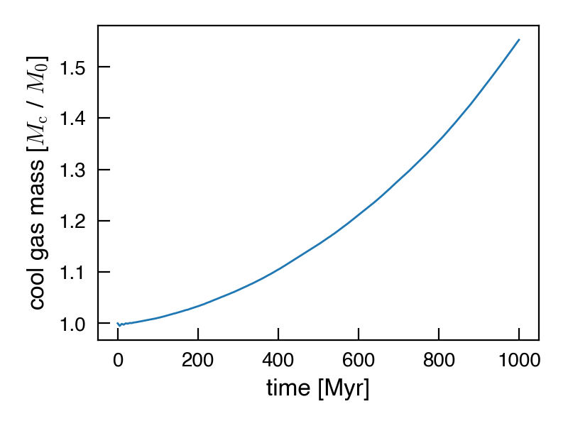
And here is a plot of the mass growth over time.