Magellanic Stream Tests

This will be the first in a series of posts dedicated to better understading the origin of gas detected in UV absorption with Magellanic Stream velocities.

First things first, simulation setups. Based on previous discussions, I tried two initial sets of ICs. The first was a standard KH setup, both in 2D and in 3D (a cylinder). I’ll only discuss the 2D version here, since I think we should use a cloud setup, instead. Perturbations were applied to the y veloicites in order to seed an instability. Boundary conditions are periodic on the x borders, and are held steady at the background state on the y boundaries.

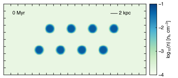
Background conditions: \(n = 1.68\times10^{-4}, \quad v_x = 0\,\mathrm{km}\,\mathrm{s}^{-1}, \quad T = 3\times10^{6}\,\mathrm{K}\)

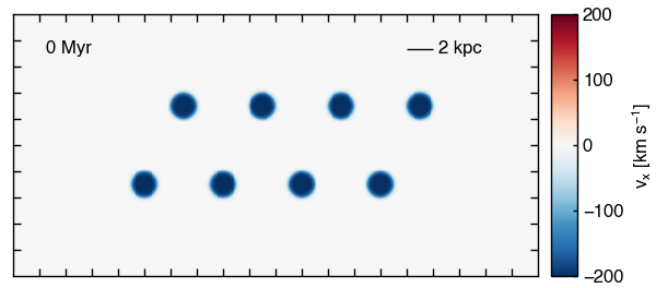
Stream conditions: \(n = 5.4\times10^{-2}, \quad v_x = -200 \,\mathrm{km}\,\mathrm{s}^{-1}, \quad T = 10^{4}\,\mathrm{K}\)

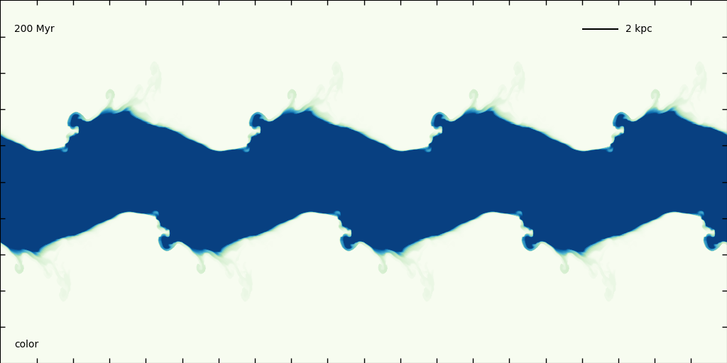
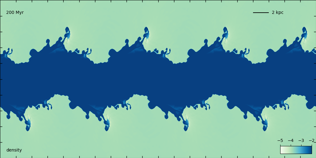
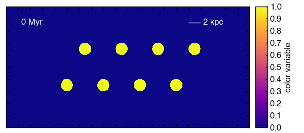
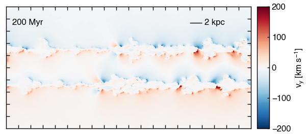
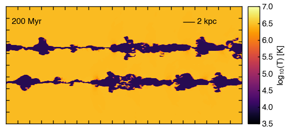
This constitutes initial pressure equilibrium between the background gas and the stream. Without pressure equilbrium, the stream will quickly either collapse or expand. For now, I’m implementing a temperature floor of \(10^{4}\,\mathrm{K}\); we may want to relax this once we’ve settled on a setup. In addition to evolving the conserved variables, I’m also evolving a color variable that traces the initial state of the gas - 0 for background material, 1 for stream material. Below are the color, density, x-velocity, y-velocity, and temperature for this setup after 200 Myr.

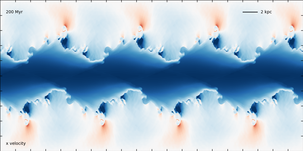
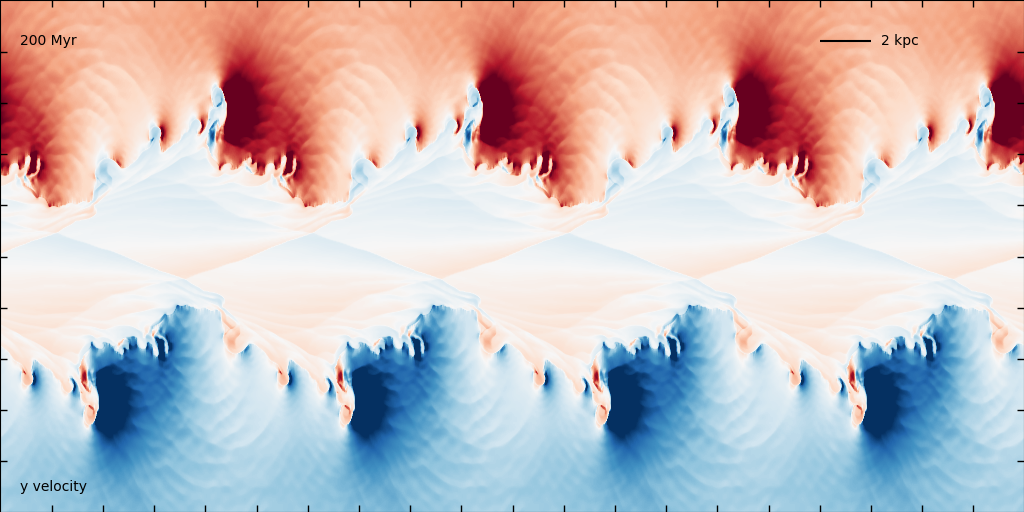
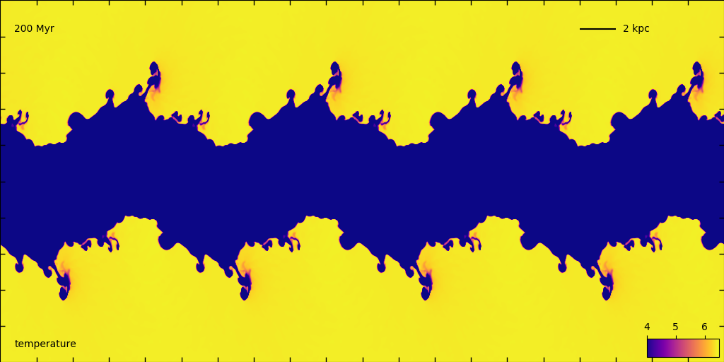
The velocities in the above plots range from -200 to 200. As you can see, the y velocities are rather extreme - this is partly a result of the 2D nature of the simulation - as the hot gas cools onto the stream, a large velocity gradient is created in the y direction. It turns out this is much less severe in the 3D case (because there is a lot more gas available).

While the original motivation for this setup is its simplicity, it turns out to have some rather significant drawbacks. One is that the total amount of gas in the stream is too large - since the stream is in reality highly fragmented, it’s difficult to have both realistic number densities and realistic spatial extent with this setup. A second is that setting up the perturbations in the 3D case is non-trivial, and a lot of decisions have to be made. For these reasons and others, I propose a different setup…

Clouds

A cloud setup is fairly straightforward, and I think will be easier to represent the current stream situation. For the clouds, I’ve done an initial test with spheres, each with a radius of 1 kpc, and the same background / interior physical variables as listed above for the KH setup. I staggered them for this run, but I think we can play with this until we get something we like.

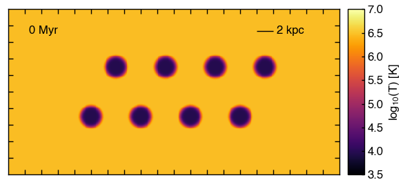
This is a 40kpc x 20 kpc box. I’ve run this setup in both 2D and 3D for 200 million years. The velocities in the 2D version are wildly different than the 3D version (for the same reason as in the KH setup), so I’m going to focus on the 3D case for the remainder of this post. Below are movies of the density and temperature projections for 200 Myr of evolution. This simulation is fairly low-res, 512 x 256 x 256 - we’ll probably want to at least double that in the end, but it currently satisfies the minimum resolution quoted by Gronke & Oh 2018 to caputure converged cloud growth from a cooling hot background (8 cells per cloud radius).

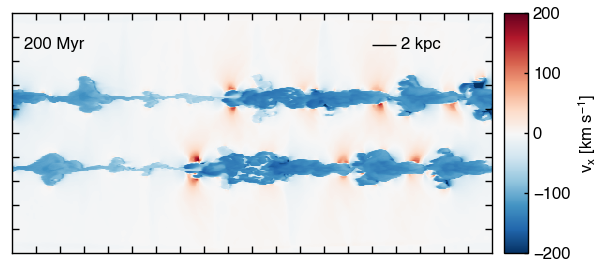
After 200 Myr, the slices look like this:

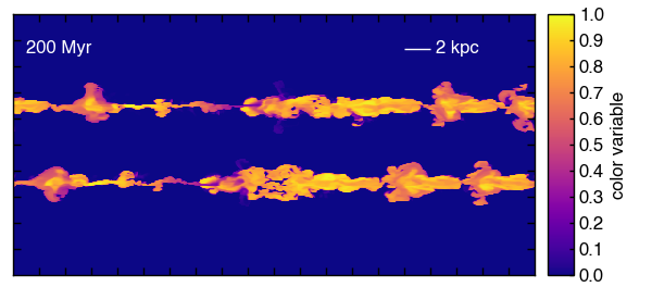
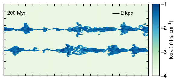
A quick calculation using the color shows that after 200 Myr there is \(3.45\times10^{7}\,M_\odot\) of cool (\(T < 5\times10^{4}\,\mathrm{K}\)) gas, of which \(8\times10^{6}\,M_\odot\) was originally hot background material (or about 20%).

I’ve also done a quick test of what a synthetic absorption line might look like. This is Si absorption for two different ions, projected in the \(z\) direction and averaged over the whole box. This means the velocities are all perturbations in the \(z\) direction, but I assume they look relatively similar to the \(y\) perturbations shown above.

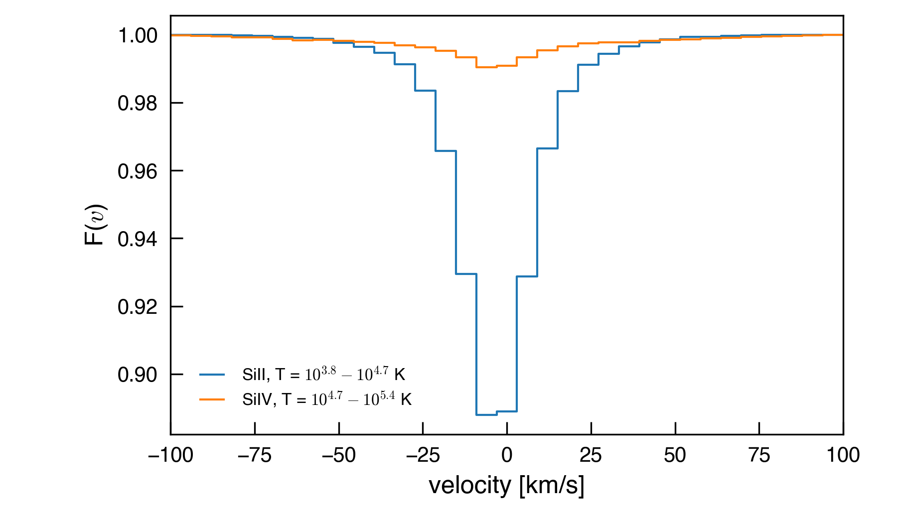
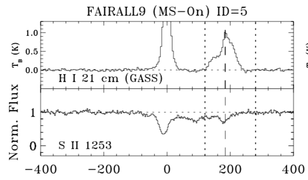
We can talk more about how I did this versus how the measurement is made, but I’m initially rather encouraged by how similar e.g. the SiII looks like to some of Andy’s measurements, for example in this figure:

Things I like about this setup:

• It’s easy to give the stream the sort of two-filament nature that is observed (Putman 2003).
• Having the clouds run into each other actually creates a nice series of density contrasts - if we allow cooling to lower temperatures, this may end up looking not dissimilar to the actual stream.
• Using spheres for the clouds will inhibit KH instabilities, as will low resolution. This then will effectively constitute a minimum constraint on how much gas could have cooled from the halo and been entrained in the stream.

Things that could be improved:

• The total mass in ionized gas is 40 times lower than Andy’s estimate at the moment. In Fox 2014, he quotes \(5\times10^{8}\,M_\odot\) in neutral gas, and three times that in ionized gas. Now, maybe my clouds are way too small. The current size is actually probably more reflective of the size of the neutral gas clouds. In order to get to \(10^{9}\,M_\odot\) in ionized gas at these number densities, I’d need clouds that are more like 3.5 kpc in radius.So, maybe I should do a run with a bigger box and bigger clouds.
• It may be worth playing around with the setup a little bit more (beyond the size of the clouds). This was just a first try to see what happens!