X-ray Profiles
January 31, 2018
In the last post, I showed soft x-ray (0.3 - 2 keV) surface brightness maps for two of my outflow simulations at \(512\times512\times1024\) (20 pc) resolution. I’ve now made the same maps for the full \(2048\times2048\times4096\) (5 pc) resolution simulations. Here they are at 60 Myr for the isotropic feedback model (adiabatic sim), and for the clustered feedback model (radiative sim):
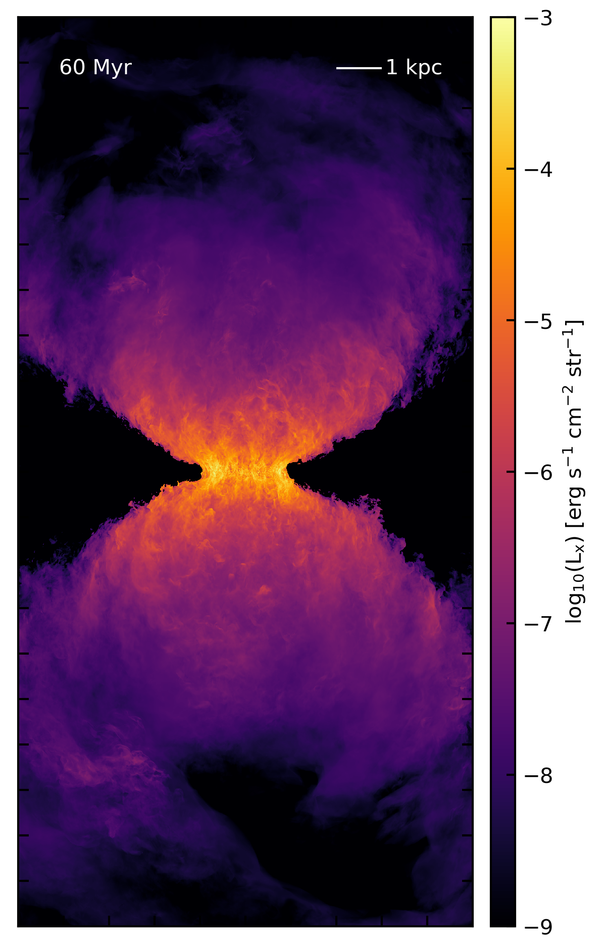
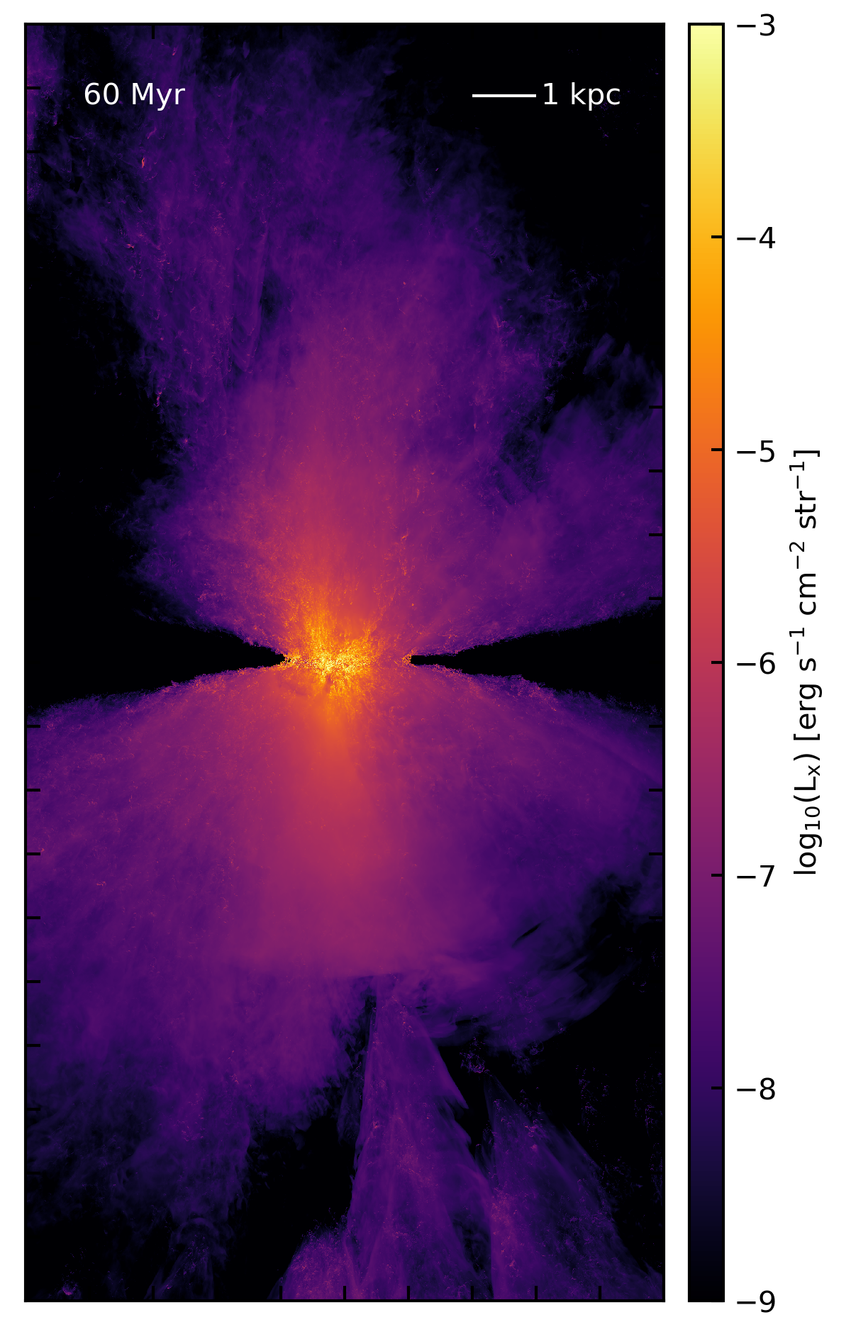
As compared to the 20 pc maps, these two plots are not so different! There’s less collimation in the clustered model, primarily because the scale height of the disk is much smaller. In the adiabatic sim, there’s no way for the disk gas to cool as shocks propagate through it, so it tends to get more and more puffed up as the simulation goes on. Both these sims show a similar vertical extent of soft x-ray emission, and filamentary and large-scale features are visible in both. In addition, the total soft x-ray luminosity is similar, \(L_x = 1.9\times10^{40}\,\mathrm{erg}\,\mathrm{s}^{-1}\) for the adiabatic sim, and \(L_x = 1.42\times10^{40}\,\mathrm{erg}\,\mathrm{s}^{-1}\) for the cluster sim. The observed soft x-ray luminosity of M82 is \(L_x = 4.3\times10^{40}\,\mathrm{erg}\,\mathrm{s}^{-1}\) (Strickland et al. 2004, Table 9).
In addition to looking at the surface brightness maps, I can also compare directly with the minor-axis surface brightness profiles derived by Strickland et al. in their 2004 paper. To create the profile, I integrate the surface brightness in slices with \(\Delta x = 10\,\mathrm{kpc}\) and \(\Delta z = 0.15625\,\mathrm{kpc}\), then divide out the area (so \(\Sigma = \int n^2 \Lambda \,\mathrm{d}x \mathrm{d}y \mathrm{d}z \,/ \int \mathrm{d}x \mathrm{d}z\)). The resulting profiles (in \(\mathrm{erg}\,\mathrm{s}^{-1}\,\mathrm{cm}^{-2}\,\mathrm{arcmin}^{-2}\)) can be directly compared with Strickland’s exponential fit for M82. In Table 6, he gives \(\Sigma_0 = 103\times10^{-9}\,\mathrm{photons}\,\mathrm{s}^{-1}\,\mathrm{cm}^{-2}\,\mathrm{arcsec}^{-2}\) with an exponential scale height of \(H_\mathrm{eff} = 0.73\,\mathrm{kpc}\). The following plots show my calculated surface brightness profiles for each of the above simulations, along with Strickland’s best fit exponential (plotted in red).
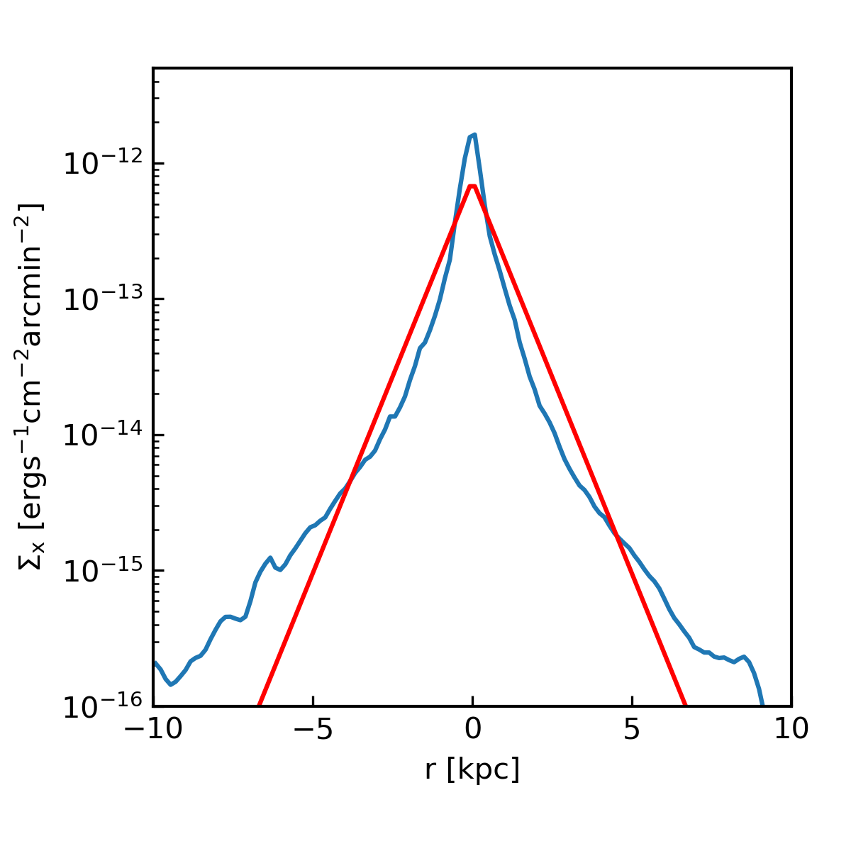
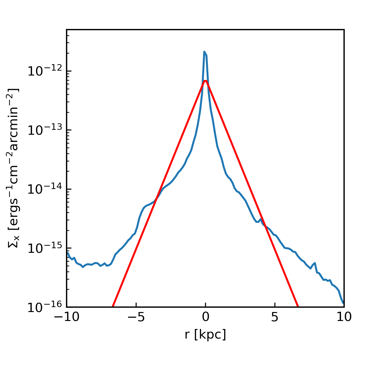
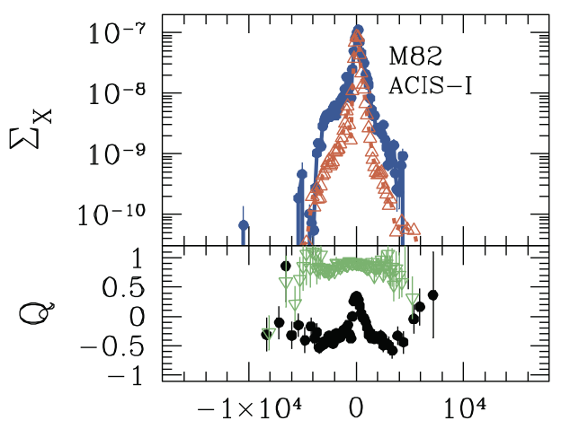
Note that I’ve converted Strickland’s data by assuming 1 photon in the 0.3 - 2 keV band is approximately \(2\times10^{-9}\) erg, as suggested in Section 4.3.2. Note also that Strickland’s exponential fit was made using only the 0.3 - 1.0 keV band data, which appear to be slightly less peaked than the 1.0 - 2.0 keV data (while my profile covers the full 0.3 - 2.0 keV band). For example, below is one of Strickland’s M82 datasets with the 0.3 - 1.0 keV data in blue and the 1.0 - 2.0 keV data in orange.
Given that, I’d say both models are looking pretty good. This has some interesting implications for the origin of the soft x-ray emission in M82, which I’ll get to in a later post.