X-ray Emission
January 29, 2018
In an attempt to connect the outflow simulations I’ve been doing to observations, I’ve decided to try to model the x-ray emission from the hot plasma and compare it to what’s seen in M82. I’ll start with a simple model for the diffuse soft x-ray emission. Briefly, for a given cell in the simulation, I’ve got a density \(\rho\), that I can convert to a number density, \(n\), by assuming that the gas is ionized, so \(n = \rho / \mu m_p\), where \(\mu = 0.6\) and \(m_p\) is the mass of a proton. Given this number density, I can also calculate a volume-averaged temperature for the gas in the cell, \(T = e (\gamma - 1.0) / n k_B\), where \(e\) is the internal energy density (tracked in the dual-energy version of Cholla), \(\gamma\) is the adiabatic index (assumed to be 5/3), and \(k_B\) is the Boltzmann constant. I can then calculate the total radiative luminosity from the cell via a cooling function \(\Lambda\).
I’ll start with the analytic cooling function that was used for these simulations, which is a fit to a CIE curve made with Cloudy assuming solar abundances. I can then create a surface brightness map for the soft X-rays by integrating \(n^2 \Lambda\) along the line of sight for a given projection in my simulation. Only cells with temperatures in the soft X-ray band are included in the integration. I convert from temperature to energy by assuming \(E = \frac{3}{2} k_B T\), as appropriate for a monatomic gas. This results in a brightness in \(\mathrm{erg}\,\mathrm{s}^{-1}\,\mathrm{cm}^{-2}\). Dividing by \(4\pi\) steradian gives a surface brightness. The resulting surfaxe brightness map for the \(512\times 512 \times 1024\) adiabatic simulation at 60 Myr with central injection feedback looks like this:
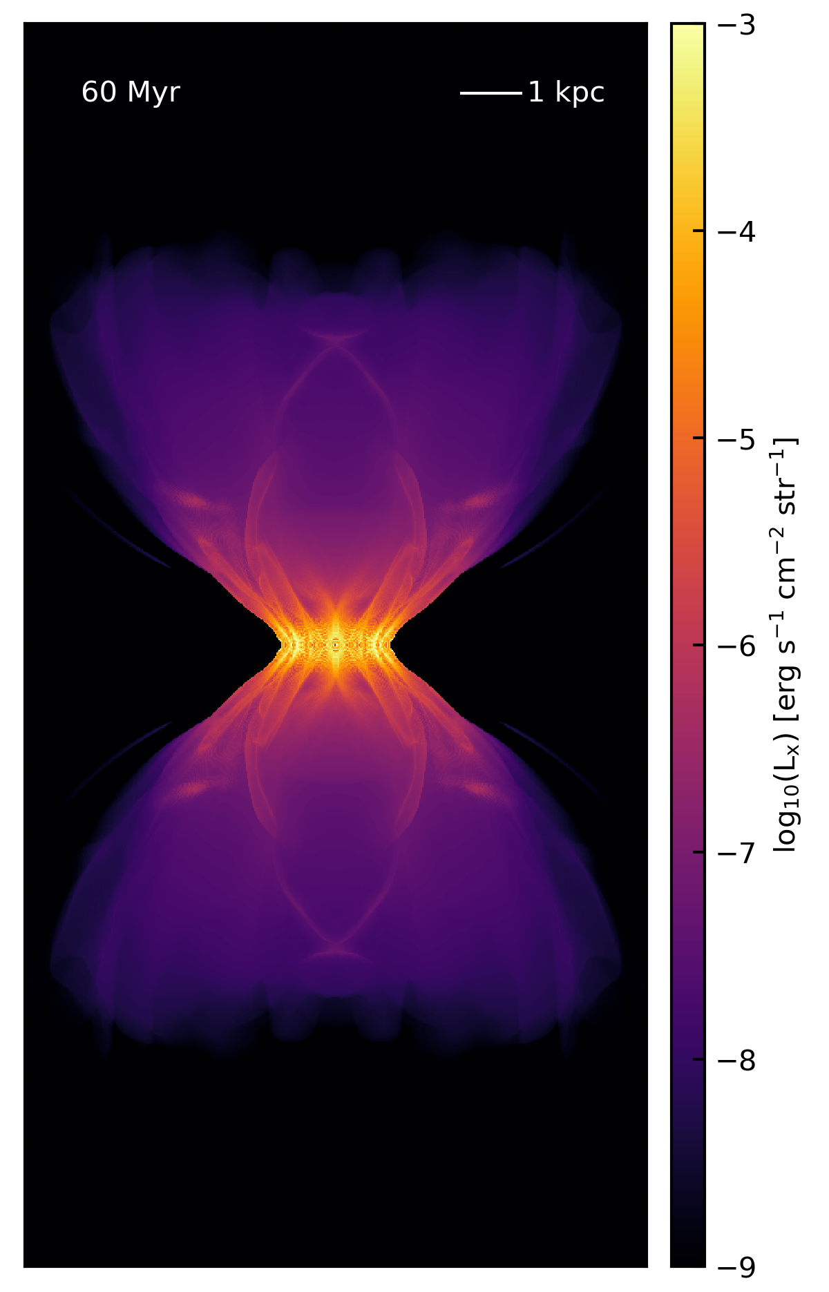
Clearly, the soft x-rays are highly collimated in this simulation. The additional features that show up in the x-ray map are from interacting shocks within the simulation volume. At this resolution, the large-scale evolution of the simulation is not yet converged. At higher resolutions, the disk-outflow interface region becomes highly turbulent, leading to more filamentary structures (figure coming soon). Interestingly, the soft X-ray luminosity integrated over the entire simulation volume is \(L_x = 2.9\times10^{40}\), which is suprisingly close to the total oberserved luminosity. For example, Strickland et al. (2004) calculate an observed diffuse soft X-ray luminosity for M82 of \(L_x = 4.3\times10^{40}\) (see their Table 9).
Here’s the surface brightness map for the 512-resolution clustered feedback simulation (which includes cooling), so is actually self-consistent:
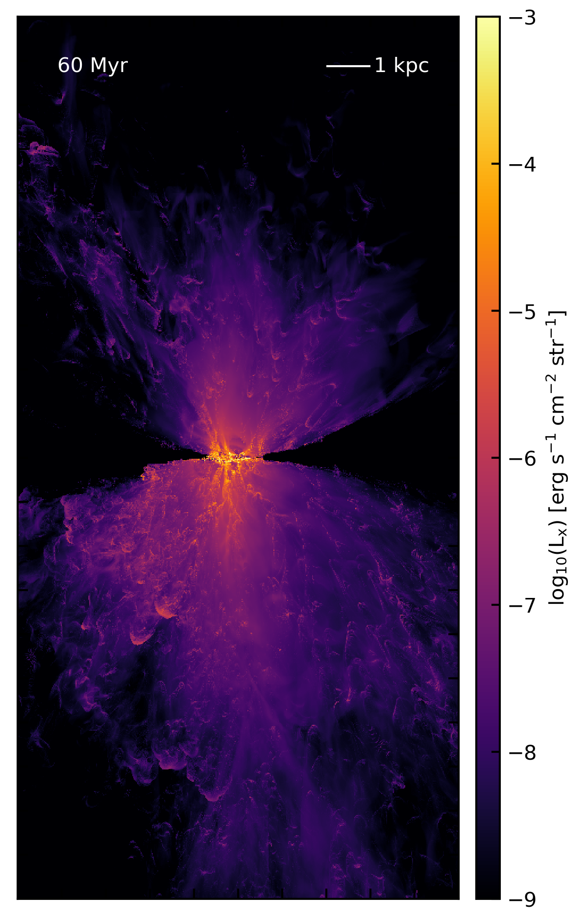
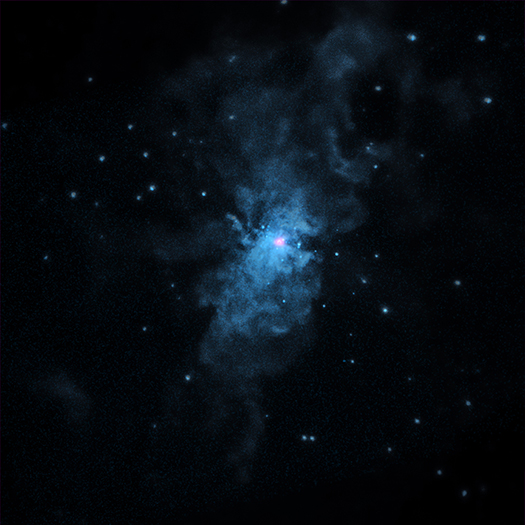
Here we see less collimation. There is also significant assymetry, with the soft X-rays extending farther in radius in the lower half of the simulation volume. The total X-ray luminosity for this simulation is lower, \(L_x = 4.5\times10^{39}\), though this is still within an order of magnitude of the observations. (Also, as noted above, these values are not converged - see the next post for results of the higher resolution simulations.) The overall morphology of the X-ray emission compares favorably to the emission seen in M82. For example, here is an image of M82 in soft X-rays made with Chandra:
In the next post I’ll explore the radial profiles of the surface brightness for the two models.