Thermal Instability

In this post, I’ll describe how I’ve set up two-phase ISM initial conditions for a future superbubble test. At present, the method mostly follows the description given in Kim & Ostriker (2015).

Thermal instability is generated in a perturbed medium when the denser regions cool faster than less dense regions. The resulting pressure difference further compresses the denser patches, which further increases the cooling rate, because cooling is proportional to the density squared. If photoelectric heating of the gas is also applied, there will be two equilibrium solutions, one in a high density cold state, and one in a low density hot state.

To create thermal instability with Cholla, I first defined a new cooling function, \(\Lambda\), and a heating rate, \(\Gamma\). The net cooling rate per unit volume, is then given by

\(\rho L = n [n \Lambda(T) - \Gamma]\),

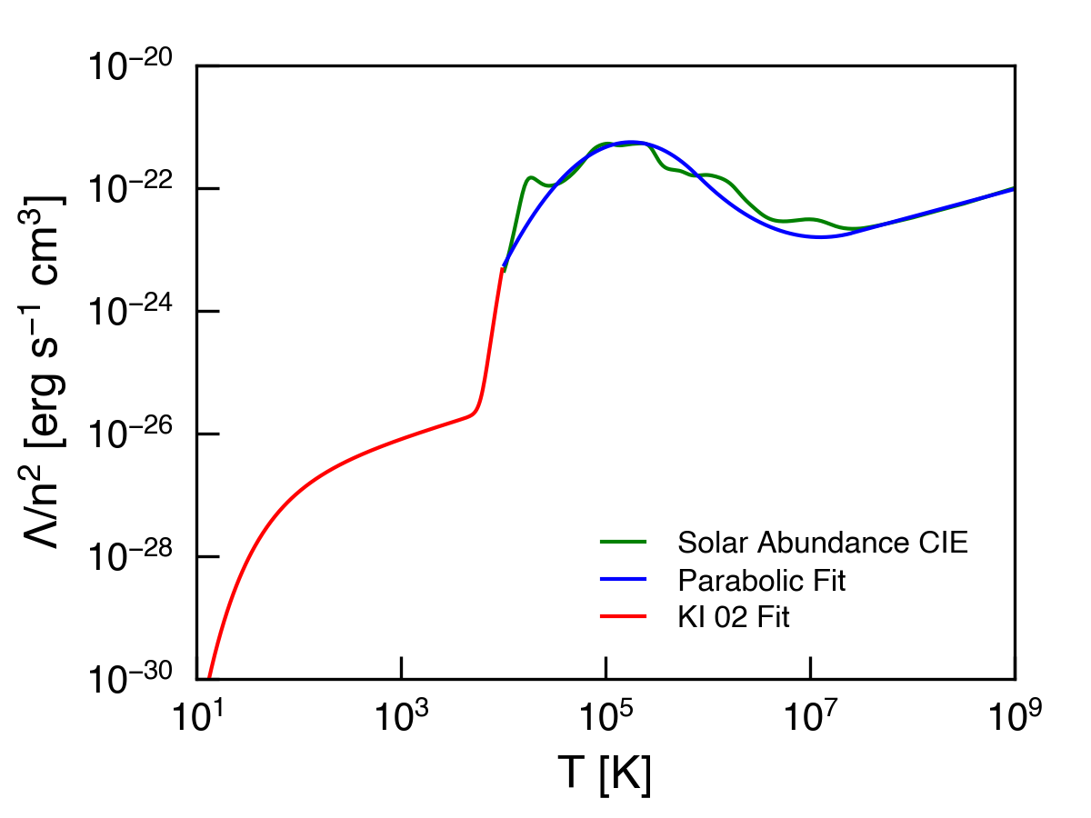
where \(n = \rho / (\mu m_\mathrm{H})\) is the number density calculated assuming \(\mu = 1.3\), as appropriate for solar metallicty neutral gas. For cooling and heating at temperatures below \(T = 10^4\) K, I use the analytic function given in Koyama & Inutsuka (2002), which includes the effects of photoelectric heating, heating an ionization by cosmic rays and X-rays, heating by \(H_2\) formation and destruction, atomic line cooling, rovibrational line cooling, and atomic and molecular collisions with grains,

\(\Lambda(T) = \Gamma\, 10^7 \mathrm{exp}\left(\frac{-114800}{T + 1000}\right) + 0.014 \sqrt{T} \mathrm{exp}\left(\frac{-92}{T}\right)\,\mathrm{cm}^{3}\),

\(\Gamma = 2 \times 10^{-26}\,\mathrm{erg}\,\mathrm{s}^{-1}\).

(Note that in their paper, the coefficient on the second term is 14, but this seems to be a typo.) At temperatures above \(10^4\) K, I use a piecewise parabolic fit to a CIE cooling function calculated with Cloudy for solar metallicty gas, and neglect heating. That function is defined in the appendix of Schneider & Robertson (2018). The combined cooling functions are plotted below:

Below 10 K, I only include heating (this improves stability of the code while the thermal instability is developing). As in previous simulations, I limit the hydro timestep such that any given cell can lose a maximum of 10% of its thermal energy in a given timestep. I also use subcyling of the cooling timestep to ensure a robust solution to the explicit integration scheme. The cooling substep is limited such that the temperature changes by 1% (or less) in a single substep.

In order to generate thermal instabilty the initial conditions must contain density perturbations. Because I am not including thermal conduction in these calculations, there will be no converged solution for a given set of perturbations. To avoid creating arbitrarily small clouds, I only perturb on modes with wavelengths of \(0.25 L_\mathrm{box}\) or longer, where \(L_\mathrm{box}\) is the length of the box. The perturbations are given by

\(\frac{\delta \rho(x,y,z)}{\rho_0} = \frac{A}{i_\mathrm{max}j_\mathrm{max}k_\mathrm{max}} \sum_{i,j,k=0}^{i,j,k = \mathrm{max}} \mathrm{sin}[x k_i + y k_j + z k_k + \theta(k_i, k_j, k_k)]\),

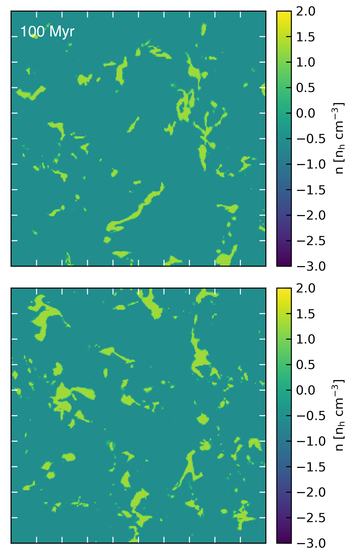
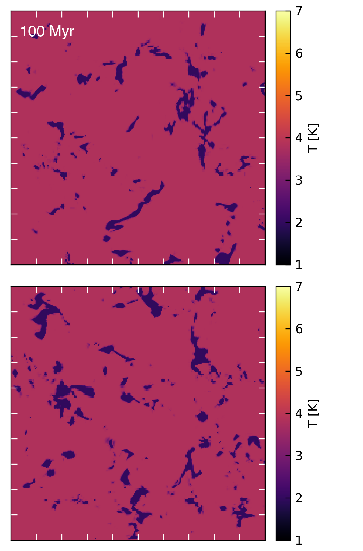
where \(k_i = 2\pi i / L_\mathrm{box}\) is the wave number, \(A\) is the amplitude of the perturbations, and \(\theta\) is a random phase. As stated above, I use \(i_\mathrm{max} = j_\mathrm{max} = k_\mathrm{max} = 4\) for the simulations in this post. I set \(\rho_0\) such that the average number density \(n = 2\), and the initial pressure \(p / k_\mathrm{B} = 2348\,\mathrm{K}\,\mathrm{cm}^{-3}\). The amplitude of the initial perturbations is 10%. Below are movies showing the development of the instability in the density and temperature projections. The box size is \(L_\mathrm{box} = 100\) pc, and the resolution is \(256^3\).

The instability is saturated by \(\sim 75\,\mathrm{Myr}\), with the mean density in the low density regions of \(n\sim 0.27\,\mathrm{cm}^{-3}\) while in the high density clouds \(n\sim 27\,\mathrm{cm}^{-3}\). The corresponding temperatures in the low and high density regions are \(T\sim 80\) K and \(T\sim 6700\) K, respectively. Density and temperature slices through the central \(z\) and \(y\) planes are shown below.