Milky Way 2D
February 15, 2017
In order to simulate galaxy outflows, we need to start with reasonable approximation of a gas disk that is stable over many rotation periods. This post begins what will be a series of tests describing the setup of such a disk. For simplicity, I’ll start with a two-dimensional simulation.
A Milky-Way-like static potential
The static potential for my disk will be based on that of the Milky Way, with a few simplifications. (I’m ignoring a bulge compenent, and artificially increasing the halo concentration to account for adiabatic contraction of the dark matter halo.) Specifically, I’ll assume an NFW halo for the dark matter:
\[\Phi(r)_{h} = - \frac{G M_{halo}}{r f(c_{vir})}\mathrm{ln}(1+x),\]where \(f(y) = \mathrm{ln}(1+y) - \frac{y}{1+y}\) and \(x = r / r_{h}\). \(r{_h}\) is the halo scale length, which I get from the halo concentration, \(c_{vir} = r_{vir} / r_{h}\), with \(c_{vir} = 20\) and \(r_{vir} = 261\) kpc. The total mass of the dark matter halo is set by the viral mass minus the disk mass, \(M_{h} = M_{vir} - M_{d}\), which I set to \(M_{vir} = 10^{12} M_{\odot}\) and \(M_{d} = 6.5\times10^{10} M_{\odot}\). (Here, \(M_{d}\) refers to the stellar disk mass). The potential of the disk follows a Kuzmin profile:
\[\Phi(r_{d}) = - \frac{G M_{d}}{(r^2 + (r_{d} + |z_d|)^2},\]where \(r_{d} = 3.5\) kpc is the disk scale length and \(z_{d} = 0.2 r_{d}\) is the disk scale height. From these potentials, I calculate the total radial acceleration in the \(z = 0\) plane (\(a_r = -\frac{\delta\Phi(r)}{\delta r}\)):
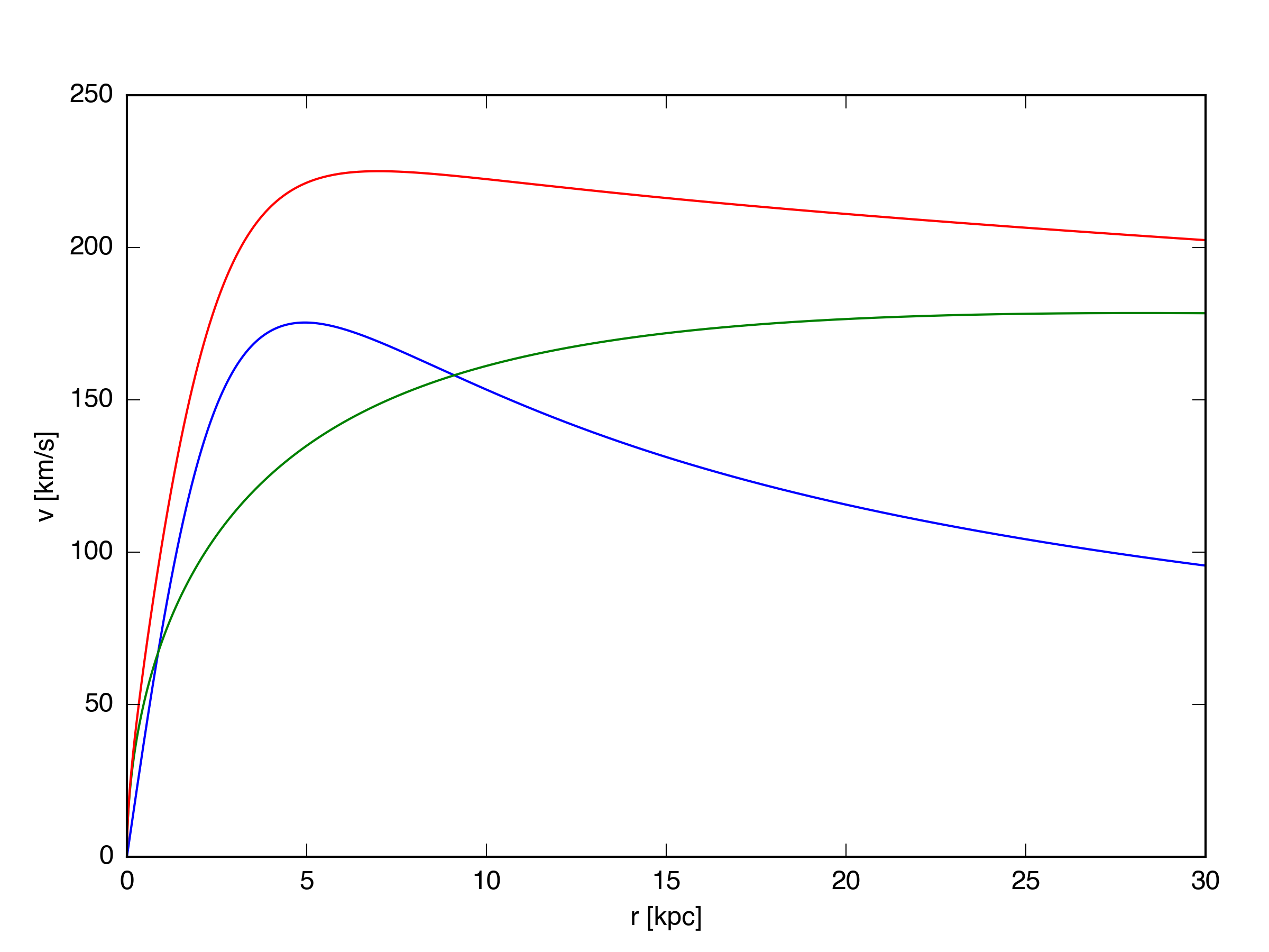
\[a(r)_{h} = \frac{G M_{h} f(x)}{f(c_{vir}) r^2},\] \[a(r)_{d} = \frac{G M_{d} r}{(r^2 + r_{d}^2)^{\frac{3}{2}}},\] \[a_{tot} = a_h + a_d.\]From the radial acceleration, I get the circular velocity due to the combined Kuzmin disk plus NFW halo profile: \(v_{c}^2 = r a_{tot}\). The circular velocity curves for this potential are shown below, with the disk component in blue, the halo component in green, and the total in red.
An Exponential Gas Disk
The potential described above gives the motion of the gas in the disk. For the disk surface density profile, I’m using an exponential, with a mass \(\frac{1}{4}\) that of the stellar disk, and a scale length \(r_{s} = 2 r_{d}\). The surface density profile thus goes as:
\[\Sigma(r) = \frac{M_{g}}{2\pi r_{s}^2} e^{-\frac{r}{r_{s}}}.\]The surface density should not evolve with time.
Results
The total circular velocity curve given above has a value of 225 km/s at a radius of 8 kpc. I’ve run the simulation for 5 orbital periods at this radius, at resolutions of \([128\times128]\), \([256\times256]\), and \([512\times512]\). Movies showing the evolution of the surface density radial profile and circular velocity radial profile are below, as well as an image of the disk (with a dot showing the approximate location of the sun).
L1 Errors
For the \([128\times128]\) grid, the L1 density error ranges between 1 and 3 percent, with an average of 2.3% over the 500 timesteps (where I’ve normalized by the average value of \(\Sigma\) across the grid. The L1 veloctiy errors are slightly better, an average of 0.21%. While the L1 errors start out lower for the higher resolution grids, the final average values aren’t that different - 1.9% and 0.18% for the \([256\times256]\) grid, and 1.5% and 0.16% for the \([512\times512]\) grid.