At some point, I’ll fill in some of the backstory from the past three months. In the meantime, here’s where things stand currently:

• We have a working equilibrium model for the Milky Way with a hot, hydrostatic halo and a rotating disk in vertical hydrostatic equilibrium that is stable for a Gyr.
• We have a working equilibrium model for M82 with the same structure.

Specific parameters for the M82 model include:

• A total disk mass of \(10^{10} \mathrm{M}_{\odot}\), derived by Greco (2012) using stellar rotation data from K-band absorption.
• A stellar disk scale length of 800 pc (Mayya 2009)
• A stellar (thin) disk scale height of 150 pc (Lim 2013)
• A virial radius of 53 kpc. This is based on the Kravstov (2013) linear fit between disk half-mass radius and halo virial radius: \(R_{\frac{1}{2}} = 0.015 R_{200}\), using disk scale length as an approximation for half-mass radius.
• A virial mass of \(5 \times 10^{10} \mathrm{M}_{\odot}\) (this is a guess, roughly based on the \(v_\mathrm{max}\)-halo mass relationship in Maller & Bullock, 2004).
• A gas disk mass of 0.25 * total disk mass, and gas disk scale length of twice the stellar disk scale length. These numbers should perhaps be adjusted, as I’ve just copied them from our MW model. Greco (2012) estimate a gas fraction of 40% for M82.

The above parameters lead to a central surface density of \(\sim 100 \mathrm{M}_{\odot} / \mathrm{pc}^2\), which is consistent with M82’s observed central surface density. M82 also contains a central stellar bar, which considerably affects the shape of the stellar rotation curve in the inner kpc. Below is my stellar rotation curve (not a fit) plotted atop the data of Greco (2012), using only the disk and halo components given above:

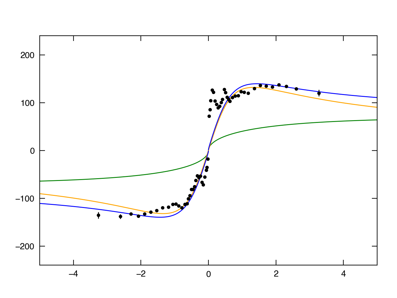
Green is the halo component, orange is the disk, and blue is the sum. The x-axis is in kpc, and the y-axis is in km/s.

The Equilibrium Model

Using Titan, I have evolved the M82 model for 400 Myr (approximately 10 rotation periods). Below are movies showing density and density-weighted temperature projections for a \(256^3\) simulation. Note that I have tapered the disk surface density to 0 between 4 and 5 kpc to alleviate an initial boundary transient. The simulation uses PPMC, the exact Riemann solver, the Van Leer integrator, and no-inflow boundary conditions.

These simulations use an adiabtic index of 5/3. In order to prevent temperatures in the disk from going below \(10^{3}\) K in the outer regions, I had to set the characteristic EOS temperature for the disk gas to \(2 \times 10^{5}\) K, which is pretty high and leads to a rather puffy disk. The characteristic temperature of the halo gas at the cooling radius is \(10^{6}\) K (I haven’t changed that from our MW model, maybe I should…).

The CC Outflow Model

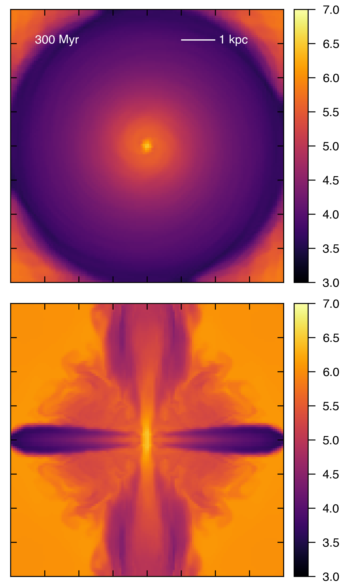
As a first test for driving an outflow, I ran a simulation exactly identical the the one above, but at each timestep, I added mass and energy according to the estimated values we used in Schneider & Robertson (2017) for the Chevalier & Clegg fit to M82. Specifically, within a spherical radius of 300 pc, I set \(\dot{M}_{\odot} = 2 M_{\odot}\) /yr, and \(\dot{E} = 10^{42}\) erg/s. I ran two versions of this simulation, one at \(128^3\) resolution and one at \(256^3\) resolution.

Density and temperature projections for the \(128^3\) simulation:

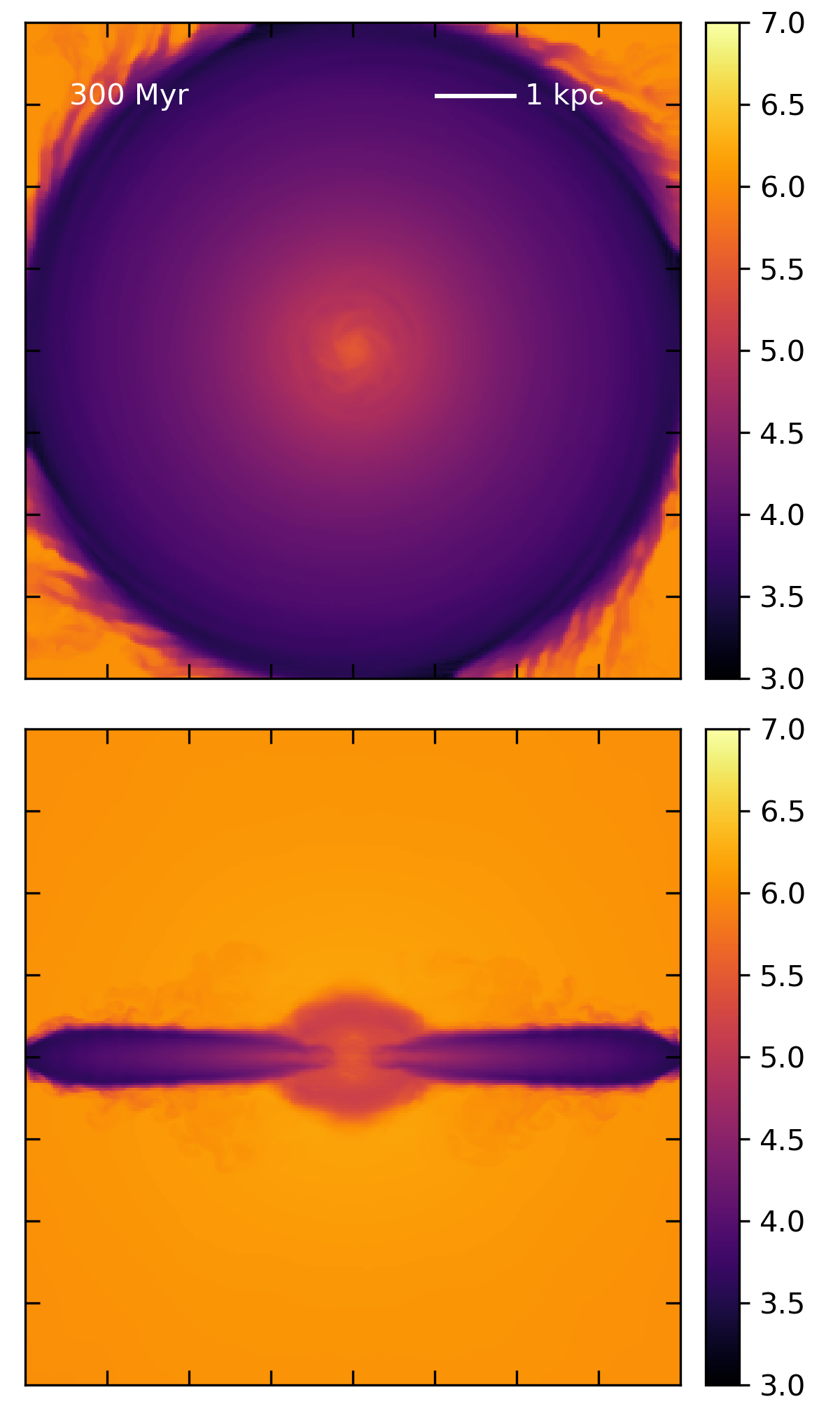
Density and temperature projections for the \(256^3\) simulation:

Only the lower resolution simulation successfully drives an outflow. This is also clearly visible in temperature slices through the central y and z planes of each simulation.

\(128^3\): \(256^3\):

Neither simulation results in the creation of very hot gas in the central starburst reason, which is presumably why driving an outflow is difficult. Perhaps I should have expected this, given that there is a large and important difference between these simulations and the Chevalier & Clegg model. CC85 assumes that the mass and thermal energy in the starburst region is set by the added mass and energy from the supernovae, while my simulation contains a large amount of gas in this region to which I’m adding the mass and energy. As a result, the gas density is much higher, and the gas would require a lot more energy to reach the temperatures predicted by the CC85 model.