Phase Diagrams

Simulation paratmeters: A sphere of radius \(R_{\mathrm{cloud}} = 5\,\mathrm{pc}\), and density \(n_h = 1.0 \,\mathrm{cm}^{-3}\) is placed in pressure equilibrium with a hot wind. The wind parameters are chosen at a distance of \(R_{*} = 1\,\mathrm{kpc}\): \(n_{wind} = 7.683798 \times 10^{-4}\,\mathrm{cm}^{-3}\), \(v_{wind} = 1.229560\,\mathrm{km}\,\mathrm{s}^{-1}\), and \(T_{wind} = 3.991611 \times 10^{6}\,\mathrm{K}\). The Mach number of the wind at this point is \(M \approx 5.25\).

Below is a snapshot showing a density projection from the \(n_h = 1\) sphere-wind simulation at 100 kyr. The dimensions of the simulation volume are \(40 \times 40 \times 150\) pc, with a cloud resolution of 32 cells / \(R_{\mathrm{cloud}}\). Numbered rectangles show regions of the simulation that will be highlighted in density-temperature phase diagrams below.

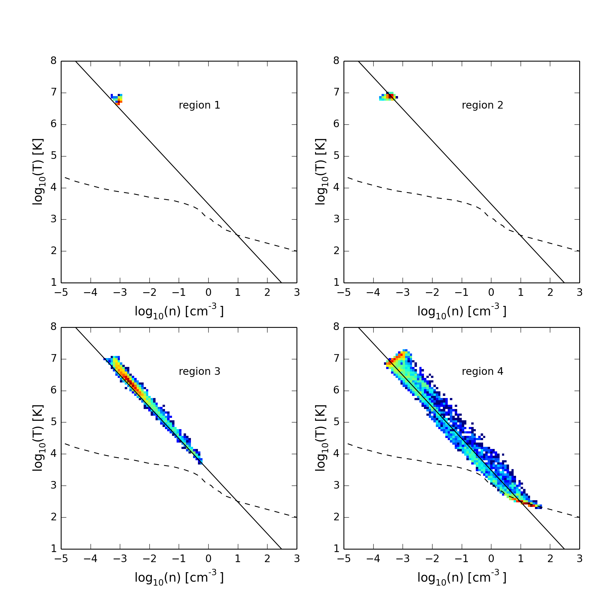
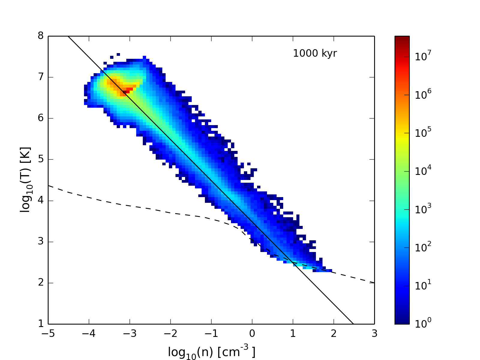
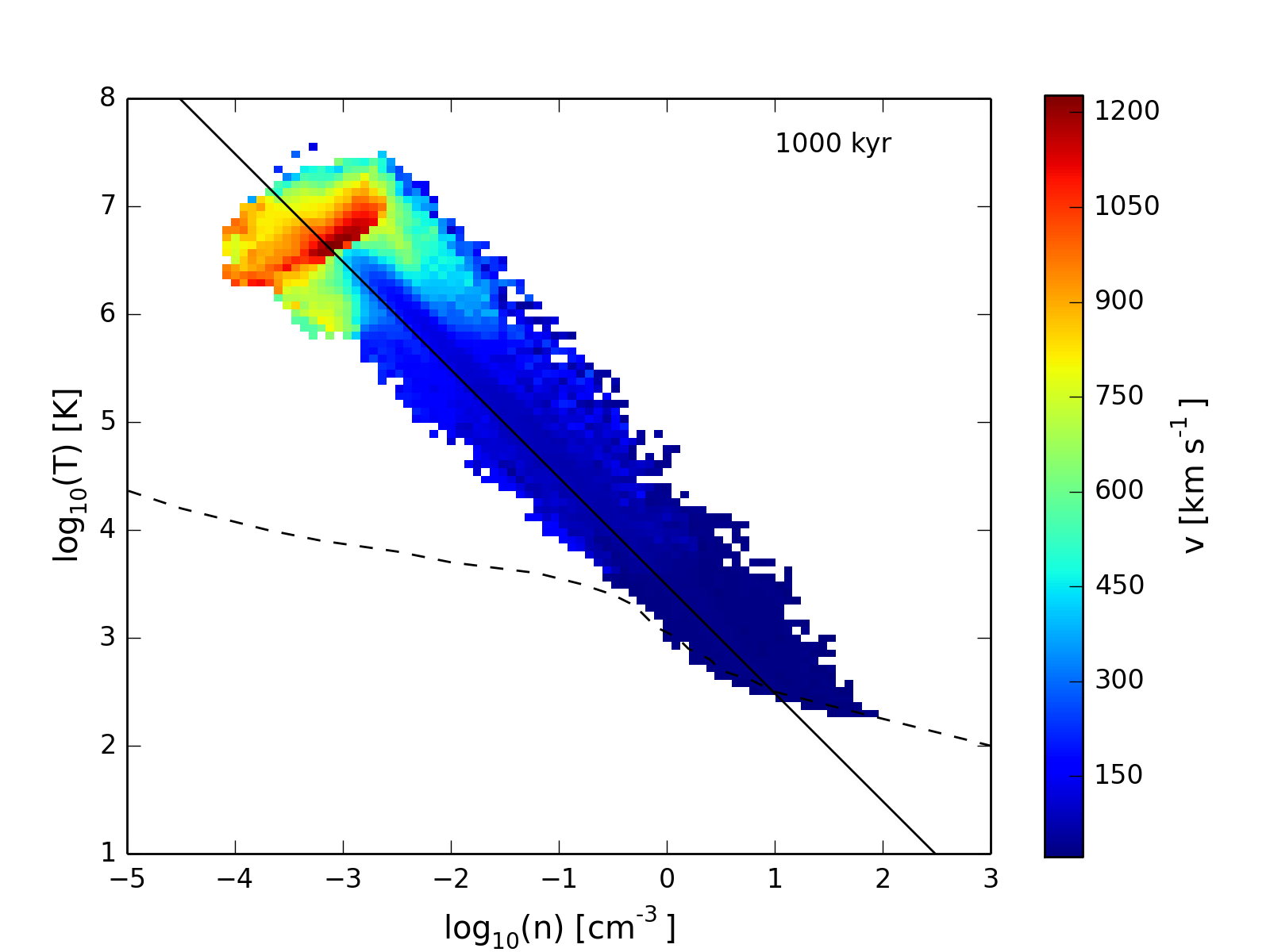
In the density-temperature phase diagrams below, in addition to the gas in the simulation volume, I have also plotted a dashed line showing where heating balances cooling in the Cloudy models, as well as a solid line showing the density-temperature relationship for an adiabatic expansion of cloud material, assuming the constant pressure set in the initial conditions.

A density-temperature phase diagram using the full simulation volume:

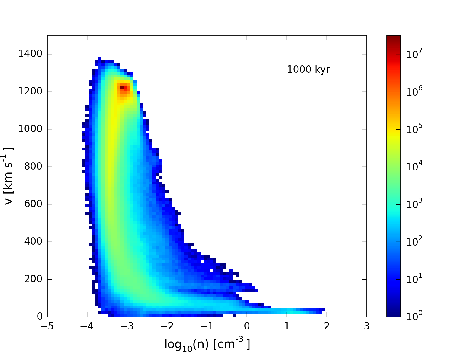
A velocity-temperature phase diagram using the full simulation volume:

A velocity-weighted density-temperature phase diagram using the full simulation volume:

In order to more clearly see how the regions of the phase diagram are populated, I have also plotted density-temperature diagrams which correspond to the regions marked on the initial snapshot (shown again here).