Mass Evolution, Part 2

This post adresses two questions: Are the simulations converged for mass evolution? How does the initial density contrast affect the mass evolution?

I attempt to answer the first question with the following plot, which shows the mass evolution as a function of cloud crushing time for the \(n_h = 1\) sphere simulation at 3 different resolutions: 16, 32, and 64 cells / \(R_{cl}\). The mass fraction is calculated as the amount of material above a given density threshold (in this case \(n = 0.05\) \(\mathrm{cm}^{-3}\)) as compared to the intial mass of the cloud.

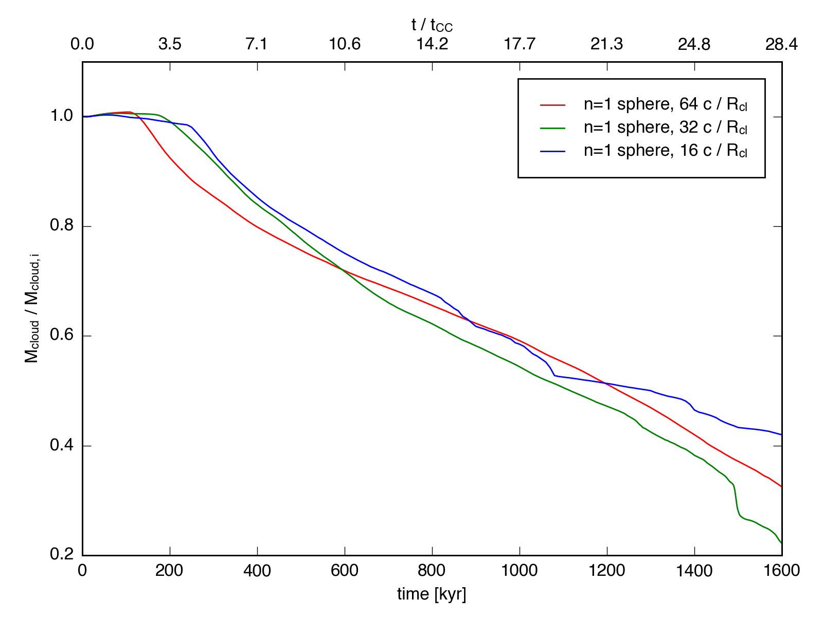
From this plot, I don’t know if we’re converged. The lines certainly aren’t lying on top of one another, nor are they approaching a common solution.

I can make the same plot using different density thresholds to measure the cloud mass, 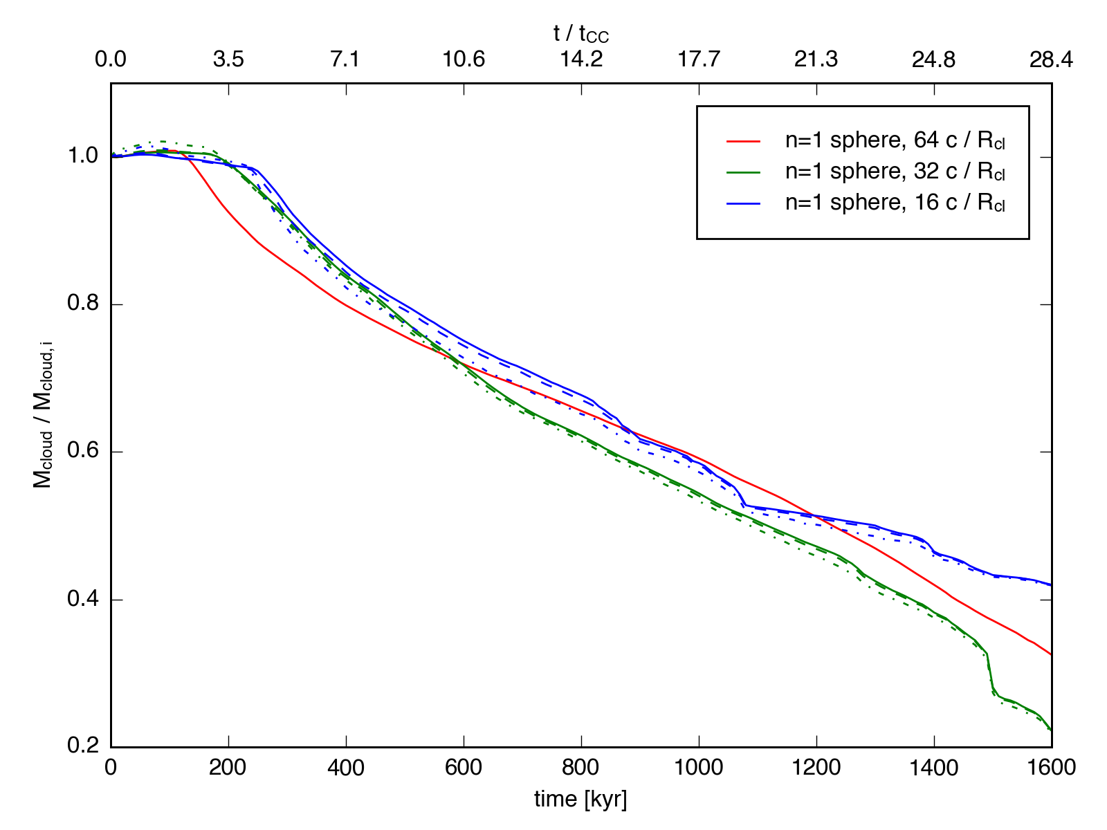but that doesn’t change the convergence much. In the plot above, the solid line represents a threshold of 1/20th the initial cloud density, while the dashed and dot-dash lines represent 1/10th and 1/3rd, respectively.

To address the second question, I plot below the mass evolution for simulations with different intial density contrasts.

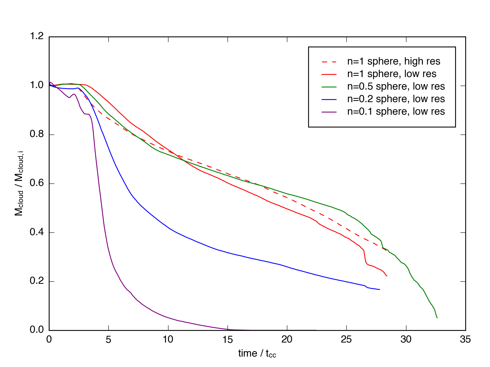
As expected, the evolution of the \(n_h = 0.2\) sphere falls between the \(n_h = 0.1\) and \(n_h = 1.0\) cases. Watching a movie of the simulation (here), we see that the \(n_h = 0.2\) cloud cools more effectively than the \(n_h = 0.1\) cloud, but it loses significantly more of its initial mass than the \(n_h =0.5\) case. To me, it looks like about half the cloud follows the adiabatic track, as indicated by the initial steep dropoff a \(t \sim 5 t_{cc}\), and the other half gets dense enough to cool and follow the radiative track.