Mass Evolution

I’ve now run low resolution (32 cells / \(R_{cloud}\)) sphere-wind simulations for spheres with mean density \(n_h = 1.0\), \(n_h = 0.5\), and \(n_h = 0.1\).

Movies of these simulations are available: n = 1, n = 0.5, and n = 0.1.

Using these simulations, we can compare the mass evolution of the clouds as a function of the cloud-crushing time. In the adiabatic regime, the evolution should be close to identical, as the density contrast should scale out (and indeed, we saw this in Table 2 of Schneider & Robertson 2015, where each cloud was mixed within 4.5 - 5 \(t_{cc}\). In the radiatively cooling regime, however, the clouds can survive much longer, if they are able to cool efficiently. We see this transition in the plot below.

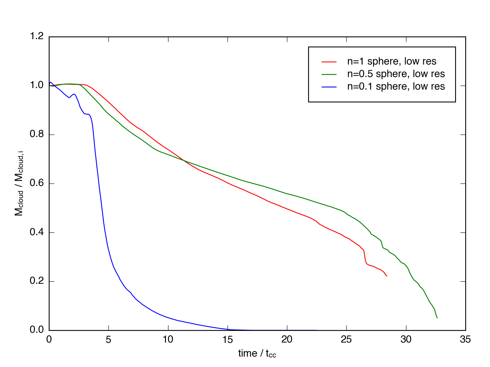
Here, the y-axis represents the fraction of the material in the simulation that is above a certain density threshold, in this case \(n = 0.05\), which is approximately \(10\times\) the hot wind density. This mass is then divided by the initial mass of the cloud, which ranges from 1 solar mass for the low density sim, to 10 solar masses for the high density sim.

We can also compare the mass evolution as a function of resolution, using the results from the low- and high-resolution \(n = 1\) simulations:

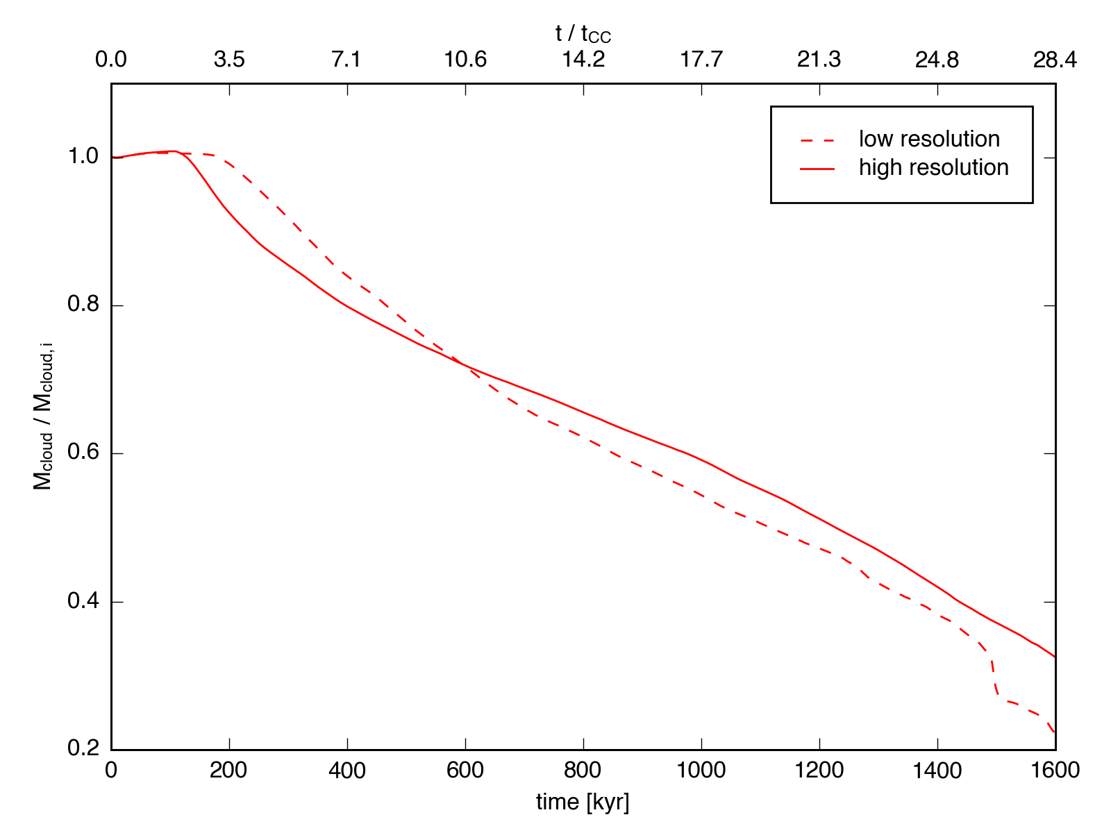
The mass evolution tracks are actually quite similar between the two, and after an initial period the low resolution cloud is actually seen to mix faster. This result contrasts the finding by Scannapieco 2015 (Figure 11), where the low resolution simulation retained a high mass fraction considerably longer than the two higher resolution comparison simulations (and this finding was used to justify the minimum resolution criterion of 64 cells / \(R_{cloud}\)). Scannapieco’s low resolution simulation showed obvious effects due to the grid; perhaps the lower courant condition used in our simulations combined with the consistent high resolution across the entire simulation volume mitigates these effects at low resolution.

Lastly, we can compare the evolution of the spherical clouds with an \(n = 1\) turbulent cloud simulation, still at low resolution, movie here. In this case, we plot the turbulent cloud as a function of cloud-crushing time calculated using the median density, rather than the average, as that was shown to match the analytic theory for spherical clouds better in Schneider & Robertson, 2015.

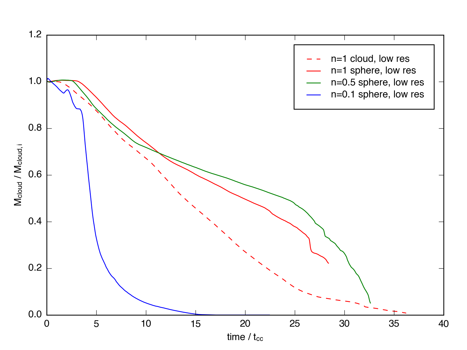
Here we find that the mixing behavior is markedly different for the turbulent cloud, even with the modified \(t_{cc}\) criterion. The evolution in the mass fraction for the turbulent cloud looks much closer to linear. This may be a result of the hierarchy of structure in the turbulent cloud leading to a much cleaner relationship for stripping and mixing material into the wind.