Cloudy Cooling in Cholla

The plot below shows cooling / heating curves generated with Cloudy for three different densities: \(n_h = 0.001\), \(n_h = 1\), and \(n_h = 1000\). Cosmic rays, the CMB, and the Haardt & Madau background (HM05) are included. The gas was assumed to have solar metallicty (GASS10).

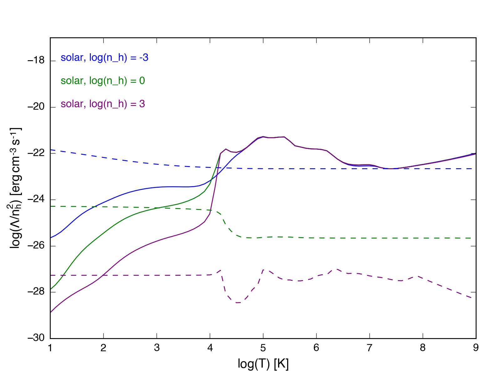
Based on these curves, a reasonable approach is to do a 2D interpolation (and include heating) for temperatures below \(10^{5}\) K. Above this temperature, only a 1D interpolation is needed to calculate the cooling rate.

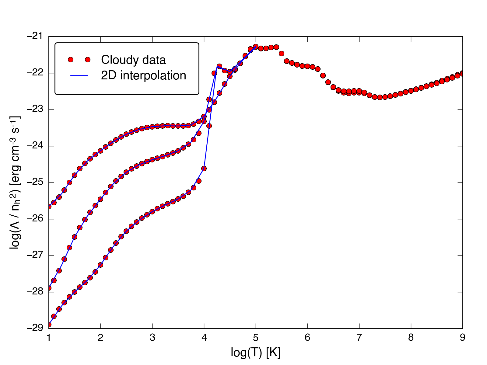
The figure below shows the results of this approach, using a standalone version of the CPU cooling function in Cholla. Below temperatures of \(10^5\) K, a 2D interpolation is done, with lookup tables calculated using Cloudy and the settings described above. The red data points shown are the same as the cooling curves in the plot above. The blue lines that appear below \(10^5\) K are the result of the 2D interpolation. Above this temperature Cholla uses the 1D spline described in a previous post.

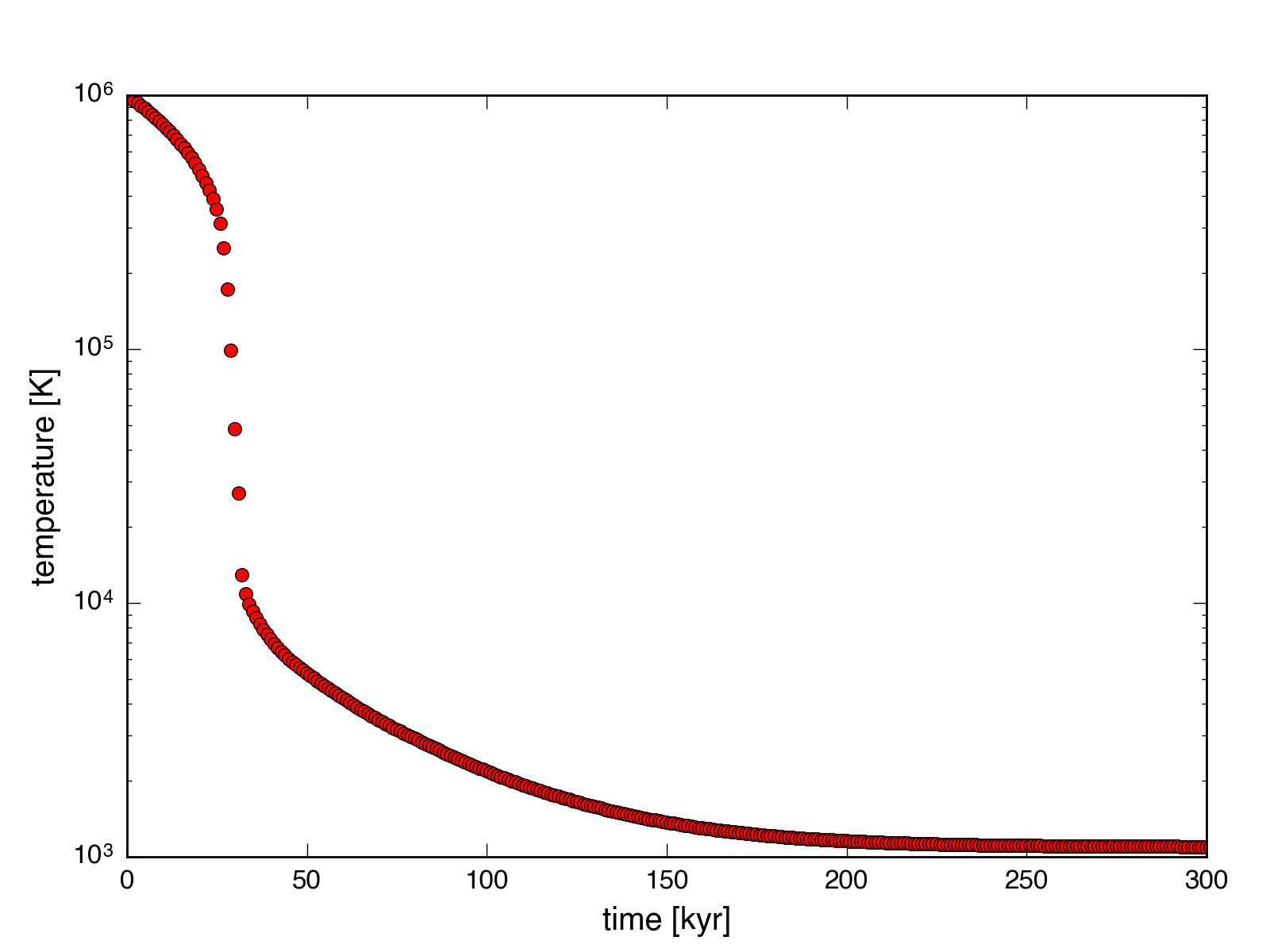
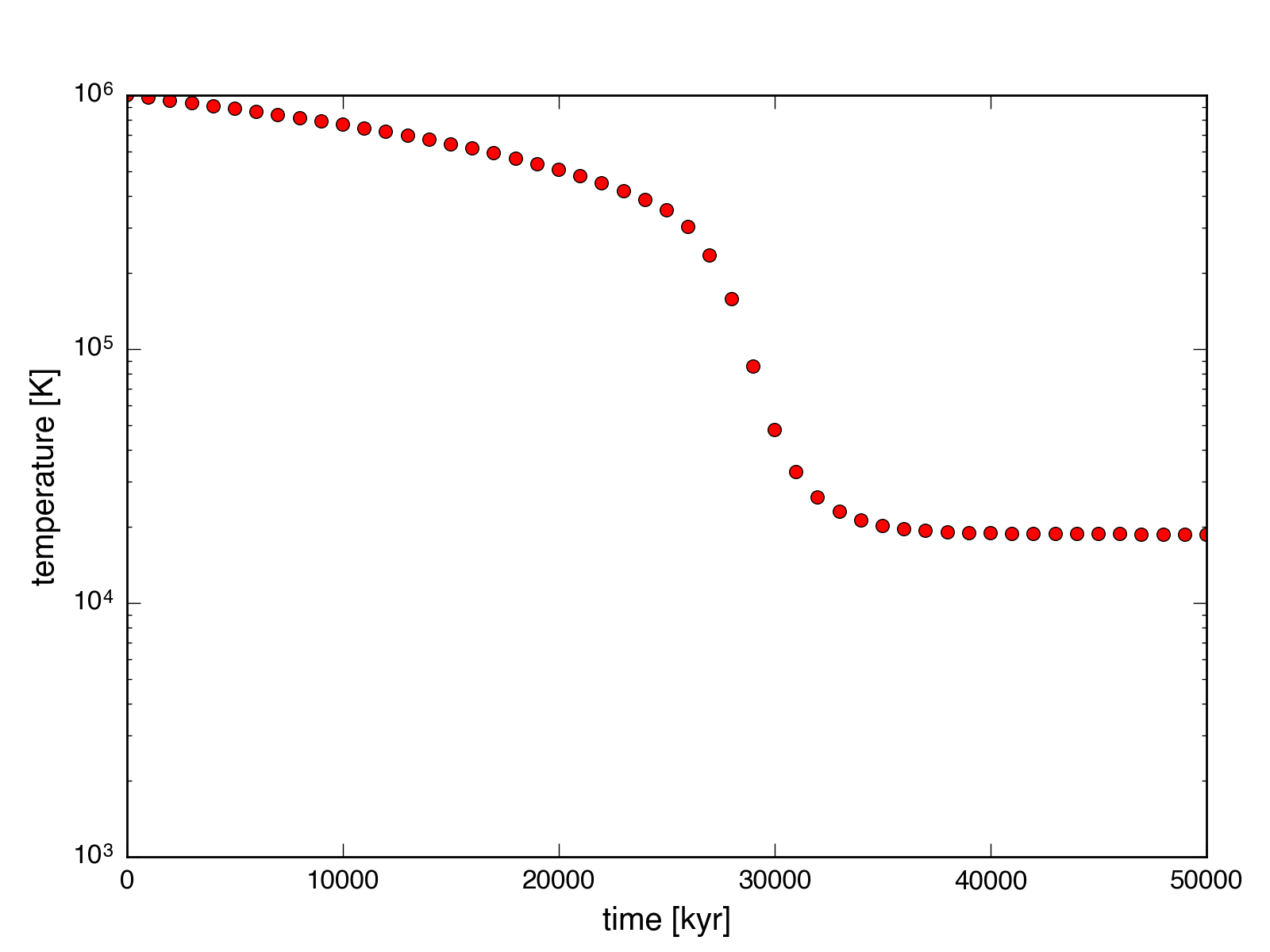
I have also tested the behavior of the cooling function in Cholla. Both the heating and cooling functions have a density dependence, with a different temperature equilibrium for gas of different densities. This behavior can be seen in the plots below, which show the temperature as a function of time for gas of two different densities, \(n_h = 1.0\) and \(n_h = 0.001\) (corresponding to the first and second plots). The higher density gas cools faster due to the \(n^2\) dependence of the cooling rate, and equilibrates at just above \(10^3\) K. The lower density gas equilibrates at a much higher temperature.